
The Depth-First Search Pattern: Exploring Trees and Graphs
How to systematically search through all paths by going as deep as possible before backtracking

Hi Friends,
Welcome to the 177th issue of the Polymathic Engineer newsletter.
This is the final article in our series on recursion. In the last article, we looked at the divide-and-conquer pattern, which breaks a problem into independent subproblems, solves each one, and combines the results. This time, we examine depth-first search, a pattern for traversing trees and graphs.
The main idea behind DFS is simple: start at a node, visit its children or neighbors recursively, and go as deep as possible before backtracking. When you reach a dead end, you return and try a different path. You keep doing this until you find what you are looking for or you run out of paths to explore.
DFS is the pattern you reach for when you need to find a path, check if something is reachable, or explore all possible paths through a structure. It works on trees, graphs, and many problems that can be represented as graphs, even if they don’t look like one at first glance.
The outline is as follows:
The Core Pattern
Finding Paths
Handling Cycles
Finding All Paths
Matrices as Implicit Graphs
When DFS Applies
Your AI shouldn’t grade its own homework

Claude Code writes beautiful code. So does Codex. But here’s the thing, they also think they write beautiful code. And when you ask an AI to review code it just wrote, you get the intellectual equivalent of a student grading their own exam. Shockingly, they always pass.
CodeRabbit CLI plugs into Claude Code and Codex as an external reviewer, different AI Agent, different architecture, 40+ static analyzers, and zero emotional attachment to the code it’s looking at. The agent writes, CodeRabbit reviews, and the agent fixes. Loop until clean.
You show up when there is actually something worth approving.
One command. Autonomous generate-review-iterate cycles. The AI still does the work. It just doesn’t get to decide if the work is good anymore.
Free tier available. Try CodeRabbit’s CLI.
Thanks to the CodeRabbit team for collaborating with me on this newsletter issue.
The Core Pattern
The simplest example of DFS is searching a binary tree to check whether it contains a particular value. We start at the root and recursively search the left and right subtrees. If we find the target value, we return true, and if we reach a null node, we return false. If either subtree contains the value, the whole tree contains it. Here is a possible way to implement this:
def contains(node, target):
    if node is None:
        return False

    if node.value == target:
        return True

    return contains(node.left, target) or contains(node.right, target)
Let’s do a quick walk-through on the following example.
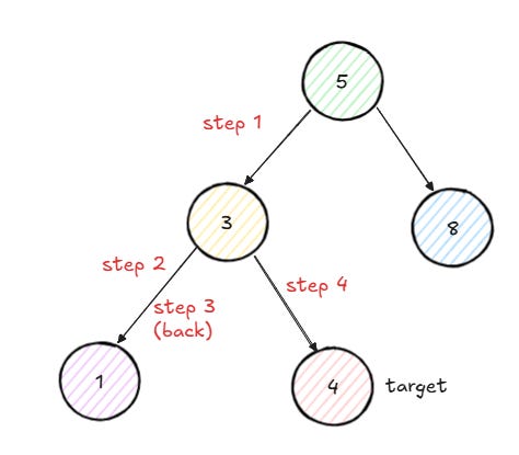
Suppose we want to find 4. We start at 5. As it is not the target, we proceed on the left subtree rooted at 3. Node 3 is not the target either, so we proceed by checking its left subtree, rooted at 1. Node 1 is not the target, and it has no children, so we return false.
We backtrack to 3 and search its right subtree rooted at 4. Node 4 is the target, so we return true. This true value propagates back up through 3 and then 5, and the function returns true.
This is the essence of DFS: go down one path as far as possible, and if you do not find what you are looking for, backtrack and try another path.
The time complexity is O(n), where n is the number of nodes in the tree. In the worst case, we go through each node until we identify the target or determine it is not there. The space complexity is also O(n) because of the recursion stack. This happens when the tree is completely imbalanced and resembles a linked list. So the depth is n.
One thing to keep in mind when analyzing tree problems is to be clear about what n represents. Here, n is the total number of nodes. If the tree were balanced, the depth would be O(log n), and the space complexity would improve accordingly.
Finding Paths
Checking whether a tree contains a value is useful, but often we need more. We would like to find the actual path from the root to the target node. This is a slight difference in how we think about the problem.
There are two approaches to do this. The first is to pass a path variable down through the recursive calls, adding nodes as we go and removing them when backtracking. The second is to build up the path as we return from the recursive calls.
I prefer the second approach. This is because at each node, we have two options as we travel down the tree: go left or go right. We do not know which way will lead us to the goal. But when we find the target and start returning, there’s only one way up. We just follow the successful path and construct the result as we go.
Here is a possible way to implement this:
def path_to_node(node, target):
    if node is None:
        return None

    if node.value == target:
        return [node.value]

    left_path = path_to_node(node.left, target)
    if left_path is not None:
        return [node.value] + left_path

    right_path = path_to_node(node.right, target)
    if right_path is not None:
        return [node.value] + right_path

    return None
The function returns None if the target is not in the subtree. Otherwise, it returns the path from the current node to the target. When the target is found, the return value is a list with just that node. As we keep returning up, each node adds itself to the front of the path.
Let’s walk through an example using the same tree as before to search for 4. We start at 5 and search the left subtree. We reach 3 and search its left subtree. We then reach 1, which has no children and is not the target, so we return None.
Back at 3, we search the right subtree. We reach 4, the target, and return [4]. Back at 3, we see that right_path is not None, so we return [3, 4]. Back at 5, we see that left_path is not None, so we return [5, 3, 4]. The path is built from the root down to the target as we return from recursive calls.
Both the time and space complexities are O(n), as for the basic containment check. We still visit each node once, and the recursion depth is at most n in an imbalanced tree.
Handling Cycles
The DFS pattern we have seen so far works on trees. But what about when we move to graphs? The main distinction is that a graph may contain cycles. If we are not careful, we could end up visiting the same node repeatedly and entering an infinite loop.
The solution is to mark all the nodes that we have already visited. We verify whether a node is in our visited set before traversing it. If it is, we skip it. If not, we add it to the set and keep exploring.
Here is how we can check if a path exists between two nodes in a graph:
def has_path(graph, source, destination, visited=None):
    if visited is None:
        visited = set()

    if source == destination:
        return True

    if source in visited:
        return False

    visited.add(source)

    for neighbor in graph[source]:
        if has_path(graph, neighbor, destination, visited):
            return True

    return False
The structure of the code is similar to what we have seen with trees. The base case is when the current node is the target. The recursive step is to try each neighbor and see if any of them leads to the destination.
The major addition is the visited set. We check whether the current node has already been visited; if so, we return false immediately. This prevents us from going in circles. Once we visit a node, we add it to the set so we do not visit it twice.
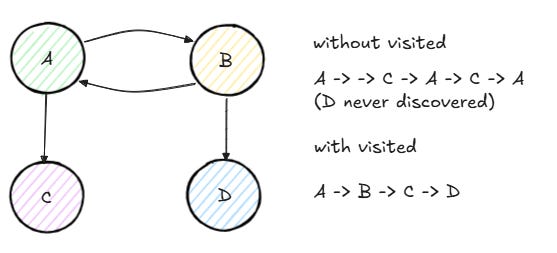
Let’s go through a quick example. Suppose we have a graph in which node A connects to nodes B and C, node B connects to nodes A and D, and node C connects to node A. We want to check if there is a path from A to D.
We start at A and add it to the visited set. We try neighbor B. We add B to visited and try its neighbor A. But A is already visited, so we skip it. We try B’s other neighbor D. Node D is the destination, so we return true. Without the visited set, we would have gone from A to B to A to B to A, forever.
The time complexity of the algorithm is O(V + E), where V is the number of vertices and E is the number of edges. Indeed, we visit each vertex at most once and examine each edge at most once. The space complexity is instead O(V) for the visited set and the recursion stack.
Finding All Paths
In the previous section, we checked whether there is a path between two nodes. But sometimes we need to find all possible paths, not just one. This requires a subtle but important change to how we handle the visited set.
When we are searching for a single path, we add a node to the visited set and leave it there. Once we know a node does not lead to the destination, there is no purpose in visiting it again. But when we are looking for all paths, different paths may share the same node. If we leave a node in visited after exploring it, other paths will not be able to use it.
The solution is backtracking. We add the node to the visited set before looking at its neighbors, then remove it when we have finished. This makes the node available for other pathways again.
Here is a possible implementation to determine all pathways between two nodes in a graph:
def all_paths(graph, source, destination, visited=None, path=None, results=None):
    if visited is None:
        visited = set()
    if path is None:
        path = []
    if results is None:
        results = []

    if source in visited:
        return results

    visited.add(source)
    path.append(source)

    if source == destination:
        results.append(path[:])
    else:
        for neighbor in graph[source]:
            all_paths(graph, neighbor, destination, visited, path, results)

    path.pop()
    visited.remove(source)

    return results
The code structure is the same as before, except for two things. First, we keep a path variable that tracks the path we are exploring. Second, after visiting all its neighbors, we delete the current node from both the visited set and the path variable.
Let’s look at an example. Suppose node A connects to nodes B and C, node B connects to node D, and node C also connects to node D. We want to find all paths from A to D.
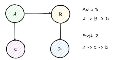
We start at A, add it to visited and path. We try neighbor B, add it to visited and path. We try B’s neighbor D, which is the destination, so we save the path [A, B, D]. We then backtrack: remove D, then remove B from the visited set and the path.
Back at A, we try neighbor C, add it to visited and path. We try C’s neighbor D, which is the destination, so we save the path [A, C, D]. We backtrack and return both paths.
The crucial point is that D is common to both paths. If we hadn’t removed B from the visited set once we had explored it, the second path through C would still work. But in a more complicated graph, failing to remove nodes would prevent us from discovering valid paths.
In the worst case, the time complexity is O(V! * V) because there could be a factorial number of paths, and each path can contain at most V nodes. The space complexity is O(V) for the recursion stack, visited set, and current path.
Matrices as Implicit Graphs
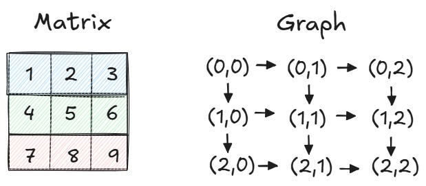
Many problems involve working with matrices instead of explicit graphs. The positive news is that we can use the same DFS pattern without explicitly converting the matrix into a graph. The graph is the matrix: nodes are cells, edges are neighboring cells.
The crucial finding is that it is straightforward to compute neighbors in a matrix. If we are at cell (i, j) and can move in four directions, the neighbors are (i+1, j), (i-1, j), (i, j+1), and (i, j-1). For some problems, you can only go right or down, so the neighbors are just (i+1, j) and (i, j+1).
Let’s now look at an example. Suppose we have a matrix of integers and want to find the path with the largest product from the top-left corner to the bottom-right corner. As the following implementation shows, we can only go down or right:
def greatest_product_path(matrix):
    rows = len(matrix)
    cols = len(matrix[0])
    result = [float('-inf')]

    def dfs(i, j, product):
        if i >= rows or j >= cols:
            return

        product *= matrix[i][j]

        if i == rows - 1 and j == cols - 1:
            result[0] = max(result[0], product)
            return

        dfs(i + 1, j, product)
        dfs(i, j + 1, product)

    dfs(0, 0, 1)
    return result[0]
The structure is the same as the DFS we have seen before. The base case checks if we have gone outside the matrix bounds. Every time we reach the bottom-right corner of the matrix, we compare the current product with the best product found so far. In the recursive step, we try both possible moves: down and right.
Notice that we do not need a visited set here. Since we can only move right or down, there is no way to revisit a cell. We will never form a cycle, so tracking visited nodes is unnecessary.
This technique can be applied to many matrix problems: path finding, path counting, determining whether a destination can be reached, etc. The matrix gives the structure, and DFS provides the exploration strategy. We just need to define what a neighbor is and what the target state is.
The time complexity is O(2^(n+m)) in the worst case, where the matrix has n rows and m columns. This is because, at each cell, we have two alternatives, and the path length is at most n + m. The space complexity is O(n + m) for the recursion stack.
When DFS Applies
DFS is the right choice when you need to explore paths across some kind of structure, whether that structure is a tree, a graph, or something that can be represented as one.
Here are some common signs that a problem calls for DFS.
The first sign is that you need to find a path or check if one exists. If the problem asks whether you can get from point A to point B, or which path you would take to arrive there, DFS is a logical fit. You explore one path at a time, moving as deep as possible before trying alternatives.
The second sign is that you need to find all paths or explore all possibilities. If there are multiple valid routes, and you need to list them, DFS combined with backtracking does the job. You explore each path fully, record it if it is valid, then backtrack and try the next one.
The third sign is that the problem involves a tree or graph structure. This covers not only explicit trees and graphs, but also implicit ones such as matrices, game states, and decision trees. If you can define what a node is and what its neighbors are, you can apply DFS.
A few more examples of classic DFS problems:
Determining if a graph is connected: start from any node and see if you can reach all others.
Finding connected components: run DFS from each unvisited node and mark all reachable nodes as part of the same component.
Detecting cycles in a graph: track nodes currently in the recursion stack and check if you revisit one.
Solving puzzles like mazes or Sudoku: explore one choice at a time, backtrack when you hit a dead end.
Computing properties of trees: height, diameter, path sums, and similar metrics often use DFS traversal.
One last thing that is worth keeping in mind is the distinction between DFS and BFS (breadth-first search). DFS goes deep along a path before going wide to explore other paths, while BFS first explores all neighbors at the current level and only then moves deeper. DFS is easier to implement recursively and uses less memory for deep, narrow structures. BFS is better when you need the shortest path in an unweighted graph.
Conclusion
DFS is one of the most flexible patterns for recursion. The basic principle is straightforward. Take one path as far as you can, and if it doesn’t get to where you want, backtrack and try another.
When it comes to trees, the pattern is simple. You traverse nodes recursively, returning results as you come back up. When dealing with graphs, you have to keep track of visited nodes to avoid cycles. In matrix problems, cells are nodes and neighboring cells are neighbors. The logic is always the same.
This brings us to the end of our series on recursion. We have covered six patterns:
Iteration: process items one at a time and collect results as you go.
Subproblems: solve a smaller version of the problem and build on it.
Selection: choose whether to include or exclude each item when creating combinations.
Ordering: determine which item comes next to produce permutations.
Divide and conquer: split the input into independent parts, solve each, and combine.
Depth-first search: explore paths by going deep before going wide.
These patterns are not mutually exclusive. Many problems combine elements of several patterns. A backtracking problem might use selection with DFS. A tree problem might use divide and conquer with subproblems. The more comfortable you become with each pattern, the easier it is to recognize which ones apply and how to combine them.
Recursion can feel tricky at first, but it becomes natural with practice. The key is to focus on two things: the base case and the recursive step. Get those right, and the rest takes care of itself.
Sir there is a mistake in the graph diagram of "Finding All Paths" section. An edge from C to D is missing because it is written "We try C’s neighbor D".