
The Divide and Conquer: Breaking Problems into Smaller Pieces
How to split a problem into independent subproblems, solve each one, and combine the results

Hi Friends,
Welcome to the 174th issue of the Polymathic Engineer newsletter.
In the last article in our series on recursion, we looked at the ordering pattern, which lets us generate all permutations of a set of items. This time, we talk about a different method: divide and conquer.
Instead of working on items one at a time, the main idea is to partition the input into multiple independent chunks, solve each separately, then combine the results.
If you have worked with algorithms, you have surely already seen divide and conquer in action. Binary search divides an array in half and searches only on the proper side. Merge sort splits an array in half, sorts both halves, and merges them back together. Tree traversals split a tree into left and right subtrees and visit each one individually.
The important thing is that we are not just taking something out and solving a smaller problem. We are breaking the input into several non-trivial subproblems and merging their solutions. That is what makes divide and conquer so powerful for some types of problems.
The outline is as follows:
The Core Pattern
Fixed Splitting: Binary Search
Trying All Splits: Unique Binary Search Trees
Other Divide and Conquer Examples
When Divide and Conquer Applies
Project-based learning is the best way to develop technical skills. CodeCrafters is an excellent platform for tackling exciting projects, such as building your own Redis, Kafka, a DNS server, SQLite, an HTTP server, or Git from scratch using your favorite programming language. Now you can also try to build your own Claude Code (for free, still in beta).
Sign up, and become a better software engineer.
The Core Pattern
The divide and conquer pattern follows three steps. First, we divide the input into two or more smaller pieces. Then, we conquer each piece by solving it recursively. Finally, we combine the results from each piece to get the solution for the original input.
This is different from what we did with the iteration and subproblems patterns. With iteration, we processed one item at a time and collected the result. With subproblems, we removed one element and solved a smaller version of the same problem. In both cases, we were reducing the input by one item.
Using divide and conquer, we partition the input into multiple nontrivial chunks. For example, if we have an array of 8 elements, we might split it into two arrays of 4. Each of those gets split into 2 arrays of 2. We keep splitting until we reach a base case, solve each base case, and then merge the results back up.
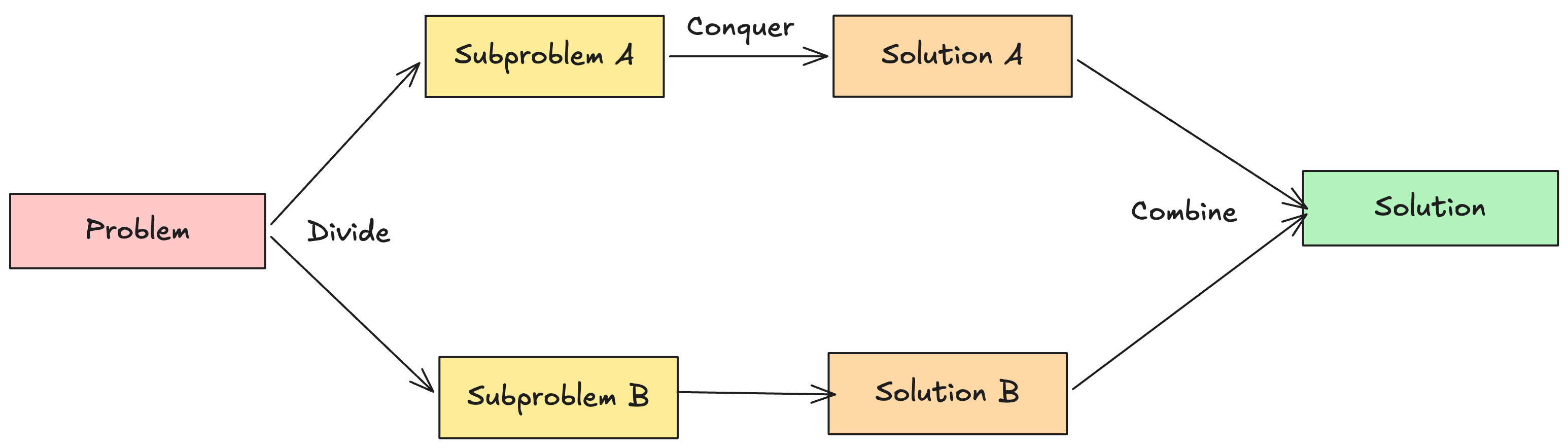
The main criterion is that the subproblems must be independent. The solution of one part should not depend on the solution of another part. This is what allows us to solve them separately and then combine the results.
There are two main variations of this pattern, depending on whether we know where to split.
In the first variation, we know exactly where to divide the input. Binary search always splits in the middle. Merge sort always divides in the middle. The split point is fixed, and the only decision is which half to look at in the case of binary search, or how to merge the halves in the case of merge sort.
In the second variation, we do not know where to split. We have to try every possible split point, solve both sides for each split, and see which one gives us the best result. This comes up in grouping problems, where we need to find all ways to partition an input or the optimal way to group elements together.
We will look at examples of both variations in the following sections.
Fixed Splitting: Binary Search
Binary search is the simplest example of a divide and conquer algorithm with a fixed split point. We always divide the array in the middle and decide which half to search based on a comparison.
The problem is straightforward: given a sorted array and a target value, check whether the target is present in the array. The brute-force approach would have to check every element, which takes O(n) time. Binary search does it in O(log n) by halving the search space at each step.
This is how the algorithm works. We examine the middle element of the array. If it is equal to the target, we are done. If the target is smaller, we search the left half. If the target is larger, we search the right half. We keep doing this until we find the target or run out of elements to check.
Here is a possible way to implement this:
def binary_search(arr, target, low, high):
    if low > high:
        return False

    mid = (low + high) // 2

    if arr[mid] == target:
        return True
    elif arr[mid] > target:
        return binary_search(arr, target, low, mid - 1)
    else:
        return binary_search(arr, target, mid + 1, high)
Let’s walk through an example to grasp how this works. Say we have the array [1, 2, 3, 5, 7, 9, 11, 13] and we are looking for 3. We start with low = 0 and high = 7. The middle index is 3, and the element at that index is 5. Since 3 is smaller than 5, we continue our search in the left half: low = 0, high = 2.
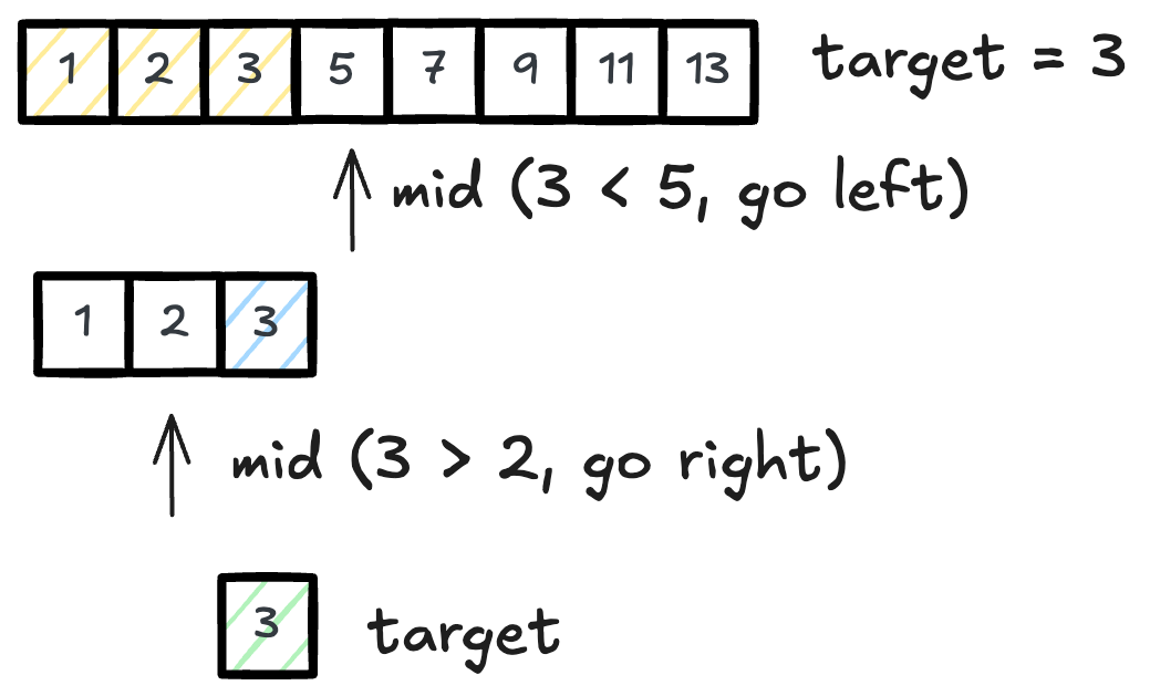
Now the middle index becomes 1, and the element there is 2. Since 3 is larger than 2, we search the right half: low = 2, high = 2. The middle index is 2, and the element at that index is the target, so we return true.
The time complexity is O(log n) because we cut the search space in half at each step. If we have 8 elements, we need at most 3 comparisons. If we have 1024 elements, at most 10 comparisons are needed. The space complexity is also O(log n) due to the recursion stack.
The crucial thing to observe is that we always know exactly where to split. No need to attempt different split points. The midpoint is always the appropriate choice, and the comparison tells us which half to search. This is why binary search is so efficient.
Trying All Splits: Unique Binary Search Trees
Now, let’s look at a problem where we do not know where to divide. Instead of always splitting in the middle, we try every possible split point and combine the results.