

Hi Friends,
Welcome to the 52nd issue of the Polymathic Engineer newsletter.
This week, we will talk about how to analyze the time complexity of a program. This potent tool allows us to evaluate how efficient an algorithm is even without running it.
Knowing about it is essential for every software engineer, not only for technical interviews but also for your daily job.
The outline will be as follows:
what is time complexity
measuring time complexity with big Oh notation
amortized analysis
Interesting Thoughts
What is time complexity
To understand how good or bad an algorithm is, we must know how it works over all the possible instances of its inputs.
In software engineering, this knowledge is usually expressed by a mathematical function known as complexity. Such a function defines the number of steps an algorithm takes for any instance size of its input.
Three interesting functions defines the behavior of an algorithm:
• The worst-case complexity, defining the maximum number of steps taken in any instance of size n.
• The best-case complexity, defining the minimum number of steps taken in any instance of size n.
• The average-case complexity of the algorithm, defining the average number of steps over all instances of size n.
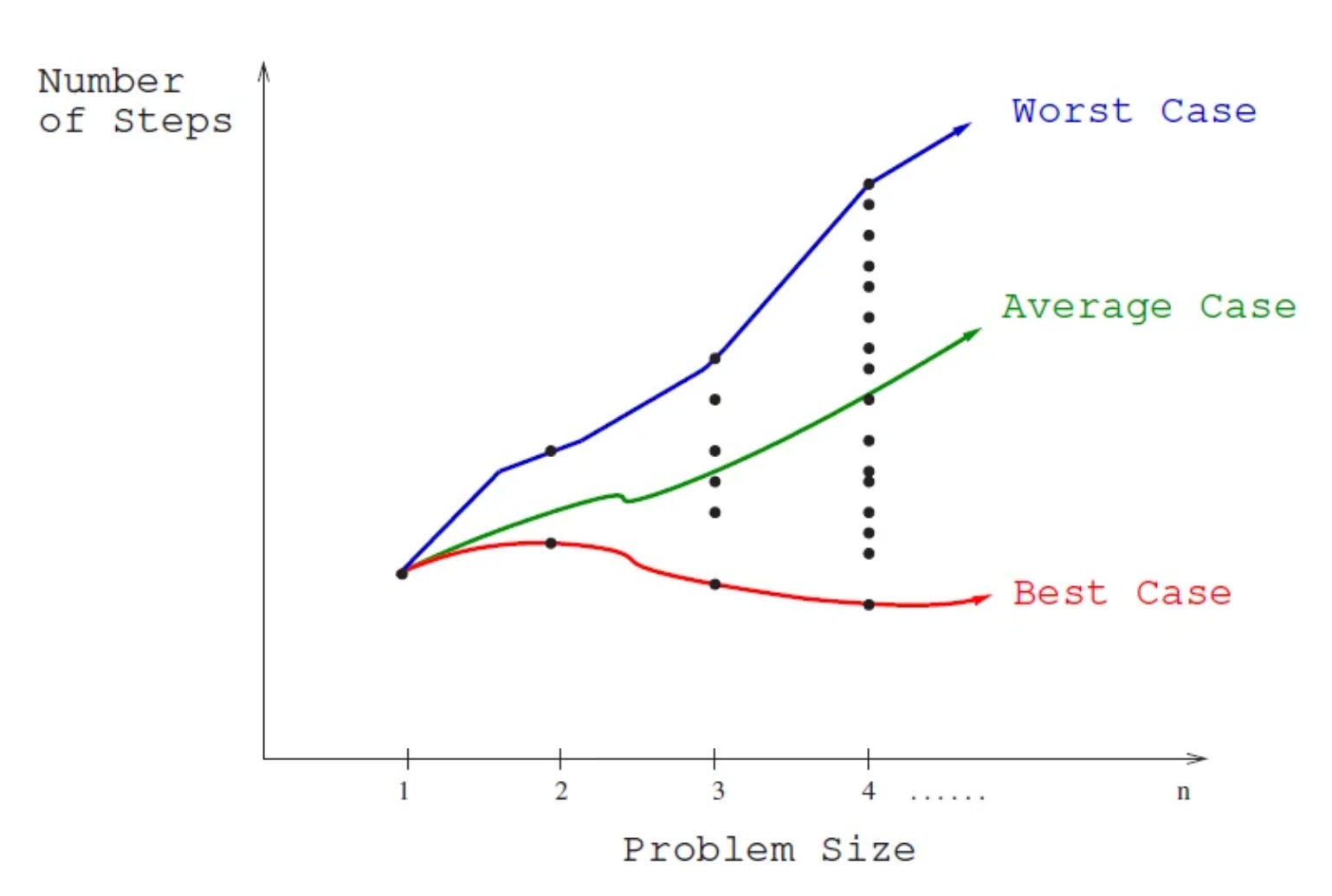
The worst-case complexity is the most useful of these three measures since it gives us guarantees about the worst possible behavior of our algorithm.
Measuring time complexity with big Oh notation
Giving a precise definition of the worst-case complexity of an algorithm requires knowing a lot of details and is often unnecessarily complex.
This is why we usually use a simplified notation that defines the worst-case complexity in terms of upper and lower bounds.
This notation is commonly called big Oh and simplifies the analysis by ignoring levels of detail that do not impact the comparison of different algorithms.
Using Big Oh notation, it is possible to group every algorithm into a finite number of classes such that two algorithms belonging to the same class can be considered equivalent.
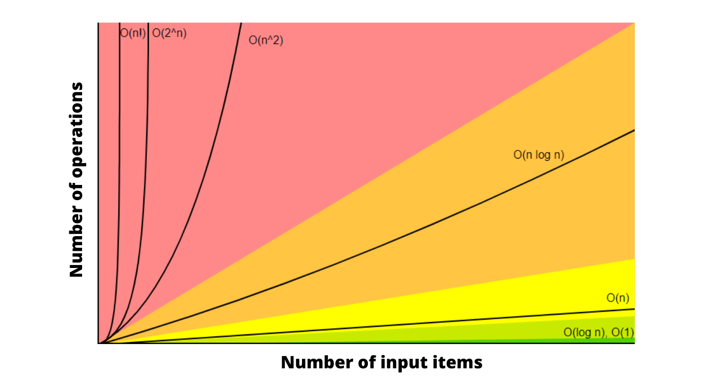
Here are the most important classes of algorithms to know:
Constant: O(1)
The running time of the algorithm is independent from the size of the input.
Example: function adding two numbers.
Logarithmic: O(logn)
The algorithm halves the size of the input at each step.
Example: binary search reduces the solution space by half after every step.
Linear: O(n)
The algorithm looks at each input item a constant number of times.
Example: a function computing the biggest or smallest item of an array.
Superlinear: O(nlogn)
The algorithm performs the following operations at each step:
split the input into two halves
execute a linear scan of the input
Example: sorting algorithms like Quicksort and Mergesort.
Quadratic: O(n^2)
The algorithm looks at most or all pairs of input items.
Example: less optimal sorting algorithms such as insertion and selection sort.
Cubic: O(n^3)
The algorithm examinates all triples of items in an array.
Example: some dynamic programming algorithms.
Exponential: O(c^n) for a constant c > 1
The algorithm uses a recursive function having a branching factor of c.
Example: a function enumerating all subsets of n items is O(2^n).
Factorial: O(n!)
The algorithm generates all permutations or orderings of the input items.
Amortized analysis
Anyway, worst-case scenarios don't happen all the time. To consider this when evaluating the performance of an algorithm, we usually use a different kind of analysis known as amortized analysis.
Suppose an algorithm is fast in most cases but slow in few. Big Oh notation only puts an upper bound on the algorithm's performance when it works slowly.
Instead, the amortized analysis approach considers that fast and slow cases happen at different rates and uses these rates to figure out how well the algorithm works on average over many runs.
It expresses that once the slow case happens, it won't happen again for so long that its cost is amortized. This approach makes sense if you want the whole set of runs, not just one, to be efficient when you run the program many times.
Let's use the dynamic array data structure to clarify this.
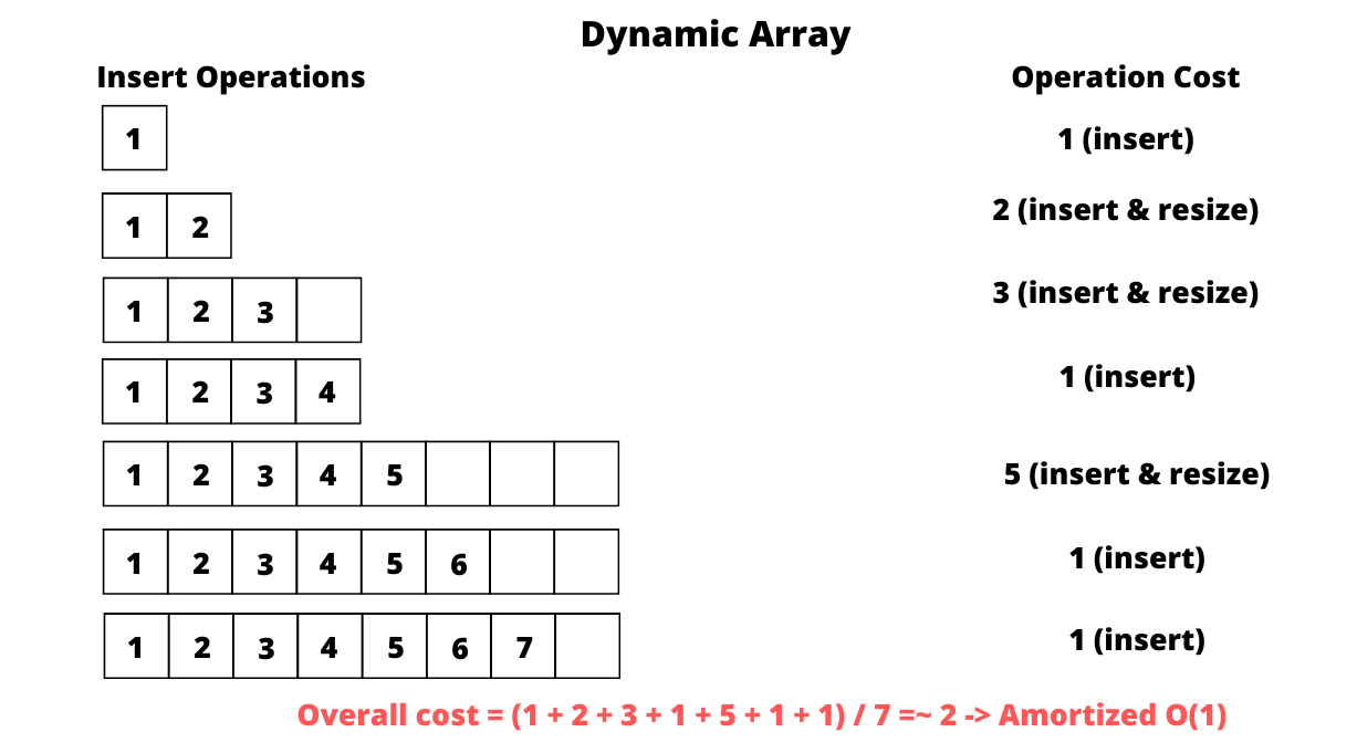
When a dynamic array becomes full, it creates a new array with double the capacity of the old array and copies all the items there.
The insert operation in a dynamic array has 2 different time complexities:
• O(1) for most of the cases
• O(n) for the few cases when the array gets full
The amortized analysis put these time complexities together.
Since the worst case happens again only after you insert half of the items, the amortized insertion of n items takes O(1). The worst-case cost of O(n) is amortized over n/2 operations.
Interesting Thoughts
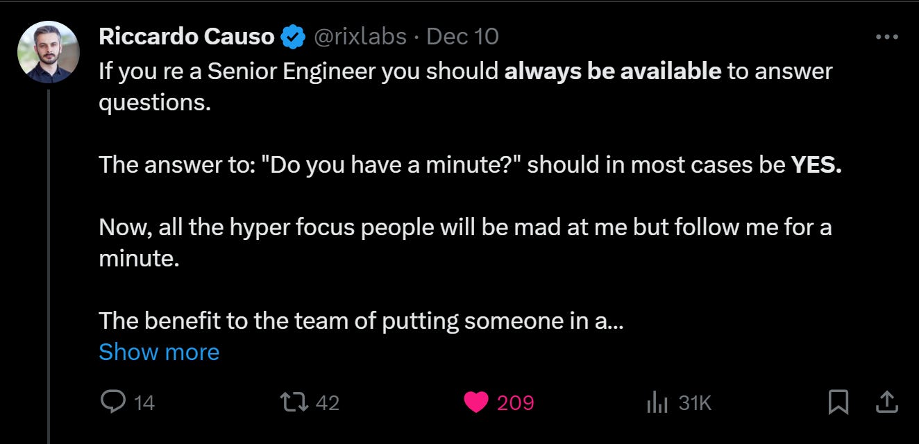
Generally, senior engineers should always be approachable and build an environment where asking questions is accepted and actively encouraged. But you can still defend your focus time, especially when the questions are not urgent. Having clear boundaries is critical.
One of the secrets to having a sustainable career as a developer is stepping away from the keyboard and taking up a hobby that has nothing to do with coding. I like to do many other things outside of coding: sports, activities with kids, reading books, and cooking are all things that help me be more productive once I go back to focusing on work.

Being transparent during interviews always pays off. But in general, admitting that you don't know something is essential for a software engineer. It makes it much easier to work with other people.