Graphs representation
A beginner friendly introduction to graphs. Different types of graphs and how to represent them.


Hi Friends,
Welcome to the 79th issue of the Polymathic Engineer newsletter. This week, we talk about graphs.
Graphs are flexible data structures that can model almost all real-world data and relationships.
For example, a graph can be used to model friendship (people are nodes, and edges connect friends), maps (cities are nodes, and edges are roads between them), or even the web (websites are nodes, and hyperlinks between them are edges).
In this issue, we will cover the basics of graphs and examine how to represent them in memory efficiently.
The outline will be as follows:
Introduction to graphs
Types of graphs
Graphs representations
Introduction to graphs
A graph is defined as a set of nodes (or vertices) V and contains a set of edges E. Each edge is an ordered or unordered pair of nodes and defines a connection between them.
From a graphical point of view, nodes are typically represented as labeled circles, and an edge between two nodes is defined as a line connecting them.
The order of a graph corresponds to the number of nodes, while the size of a graph is the number of edges. The degree of a node is the number of incident edges.
An isolated node is not connected to any other node in the graph (has degree 0), while two nodes connected by an edge are said to be adjacent.
An edge (u, v) between two nodes, u and v, can be undirected, directed, weighted, or unweighted. Each type of edge determines a different kind of graph.
Types of graphs
The first thing to remember is the distinction between undirected and directed graphs.
A graph is undirected if all its edges are unordered: an edge (u, v) also implies that the edge (v, u) exists. If this property is not valid, the graph is directed.
For example, road connections between cities are typically undirected since roads usually have lanes in both directions. Instead, a graph representing a social network is generally directed since you can follow a person, but that person may not follow you back.
A second important distinction is between weighted and unweighted graphs. Each edge (or node) in a weighted graph G has been assigned a numerical value or weight.
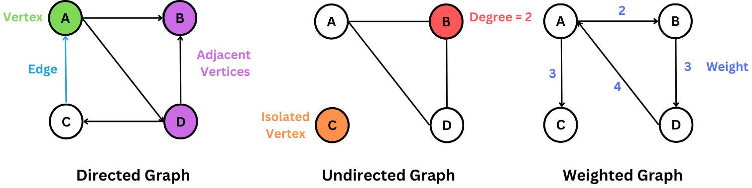
For example, depending on the specific application, road connections between cities might be weighted by length, drive time, or speed limit. Unweighted graphs have no cost distinction between various edges and nodes.
The difference between weighted and unweighted graphs becomes critical in finding the shortest path between two nodes.
In unweighted graphs, the shortest path has the fewest edges and can be found using the Breadth First Search algorithm. In weighted graphs, the shortest path may differ and needs more sophisticated algorithms like Dijkstra to be found.
It is worth mentioning two other distinctions between graphs: sparse vs. dense and cyclic vs. acyclic.
A graph is sparse when only a tiny fraction of the node pairs have edges connecting them. Graphs where a significant fraction of the vertex pairs define edges are called dense.
There is no clear boundary between what is called sparse and what is called dense, but usually, dense graphs are quadratic in size, while sparse graphs are linear in size.
A graph is acyclic if it does not contain cycles from one node back to the same node. Trees are connected, acyclic undirected graphs.
Directed acyclic graphs (DAGs) are significant since they arise naturally in scheduling problems: a directed edge (u, v) indicates that an activity must happen before v.
The topological sorting algorithm can order the nodes of a DAG to respect these precedence constraints.
Graphs Representation
Different kinds of data structures can represent a graph in memory. The most popular ones are the adjacency matrix, adjacency list, and edge list.
Selecting the right one can enormously impact performance, so it's essential to know how they work and their advantages and disadvantages.
An adjacency matrix represents a graph using a 2D n × n matrix M, where n is the number of nodes. The idea is that the cell M[i][j] represents the edge weight of going from node i to j or is 0 if no edge connects the two nodes. The weight is always 1 for undirected graphs.
The main advantage of this representation is that inserting and deleting an edge or looking up an edge weight are all operations that can be done in constant time.
However, an adjacency matrix always takes a quadratic amount of space in the number of nodes, and iterating over all the edges is an O(V^2) operation regardless of their number.
For this reason, the adjacency matrix is more suitable for dense graphs where most pairs of nodes are connected by an edge and not for spare graphs.
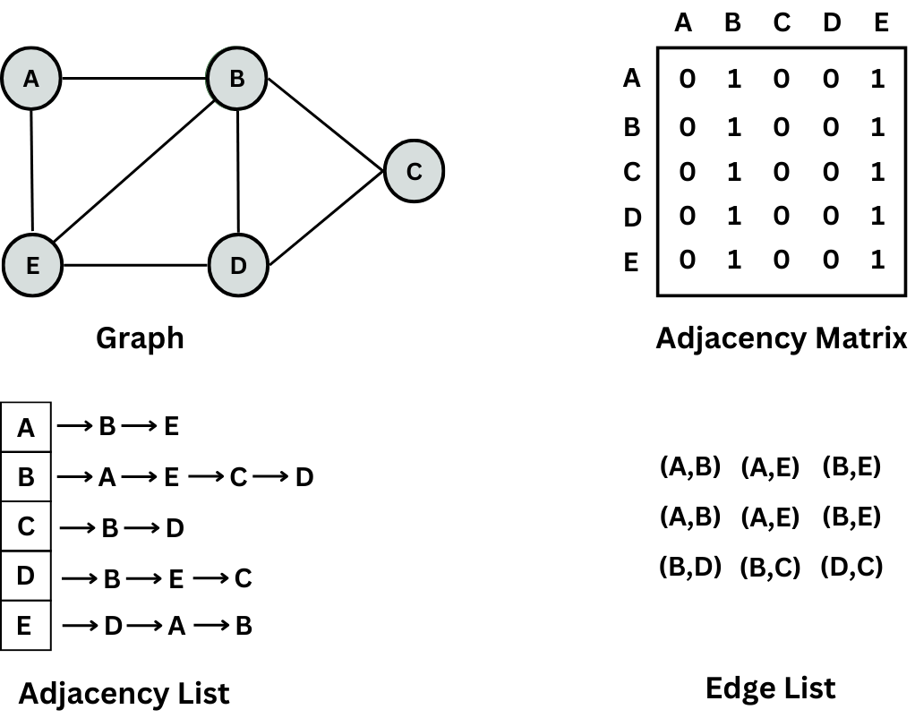
An adjacency list represents a graph as a map, where each key is a node, and the value associated with a key is a list of all the incident edges.
This representation is more space-efficient and suitable for sparse graphs since the required memory is linear in the number of nodes and edges. Also, iterating over all the edges requires O(V + E) time.
However, looking for an edge is more time-consuming since you have to search through the appropriate list to find the edge. The good news is that most graph algorithms don’t need such queries, and adjacency lists are the proper data structure for most graph applications.
An edge list represents a graph simply as an unordered list of edges. For weighted graphs, edges are defined using a triplet (u, v, w), meaning that the cost from node u to node v is w.
This third representation for graphs takes only O(E) space in memory, and iterating over all the possible edges is also a linear time operation. However, edge lists are much less used than adjacency lists since finding a node's incident edges takes time.
Before we finish our discussion, it is worth mentioning that certain graphs are not explicitly constructed using one of the above representations and then traversed. Instead, they are built as you use them without a whole in-memory representation.
For example, a state machine implicitly defines a graph where each vertex represents one of the possible states, and each edge represents a move from one state to another.
class Graph:
    def __init__(self, num_vertices):
        self.num_vertices = num_vertices
        self.adjacency_matrix = [[0]*num_vertices for _ in range(num_vertices)]
        self.adjacency_list = [[] for _ in range(num_vertices)]
        self.edge_list = []

    # Assuming it's an undirected graph
    def add_edge(self, u, v):
        # Update adjacency matrix
        self.adjacency_matrix[u][v] = 1
        self.adjacency_matrix[v][u] = 1

        # Update adjacency list
        self.adjacency_list[u].append(v)
        self.adjacency_list[v].append(u)

        # Update edge list
        self.edge_list.append((u, v))

    def display_adjacency_matrix(self):
        print("Adjacency Matrix:")
        for row in self.adjacency_matrix:
            print(row)

    def display_adjacency_list(self):
        print("Adjacency List:")
        for index, neighbors in enumerate(self.adjacency_list):
            print(f"{index}: {neighbors}")

    def display_edge_list(self):
        print("Edge List:")
        print(self.edge_list)

# Create a graph with 5 vertices
graph = Graph(5)

# Add some edges
graph.add_edge(0, 1)
graph.add_edge(0, 4)
graph.add_edge(1, 2)
graph.add_edge(1, 3)
graph.add_edge(2, 3)
graph.add_edge(3, 4)

# Display the graph representations
graph.display_adjacency_matrix()
graph.display_adjacency_list()
graph.display_edge_list()
Food for thoughts
Many people keep asking me how to improve at Leetcode, and I always suggest a similar approach. Start with easy-difficulty problems initially and build your muscles to coding basic stuff. When you can solve most of such problems very quickly and comfortably, move on to medium problems.
People saying that AI will replace software engineers either do not understand AI or do not understand software engineering. Using a natural language prompt to write code is just another abstraction layer to do more with less.

I'd try to understand how often this is expected in such a situation. Working regularly overtime is a sign of a problem with resources or expectations. No team can sustainably work like that.