Fundamental Graph Algorithms - Part II: DFS

Depth First Search and its applications on undirected graphs: finding cycles and articulation vertices.

Hi Friends,

Welcome to the 151st issue of the Polymathic Engineer.

This week, we’ll continue our discussion about fundamental graph algorithms. While we discussed Breadth-first search in the last issue, this article covers DFS. Depth-first search takes a different approach to graph traversal.

Instead of looking at neighbors level by level like BFS, DFS goes as deep as possible along each path before backtracking. If BFS is like ripples spreading across a pond, DFS is more like going through a maze by always taking the first unexplored path.

The outline will be as follows:

• Basic concepts

• Key Properties

• Implementation

• Cycle detection

• Articulation vertices

---

Project-based learning is the best way to develop technical skills. CodeCrafters is an excellent platform for tackling exciting projects, such as building your own Redis, Kafka, a DNS server, SQLite, or Git from scratch.

Sign up, and become a better software engineer.

---

Basic Concepts

The main difference between BFS and DFS is the data structure used to keep track of the discovered, but not yet processed, vertices. BFS uses a queue, while DFS utilizes a stack. However, the beauty of DFS is that you don’t need to use an explicit stack, but you can leverage recursion to get a simple yet elegant implementation.

The algorithm is straightforward. You start by choosing an initial vertex, and then you repeat these steps:

• Mark the current vertex as discovered

• Process the vertex if needed

• For each neighbor of the current vertex:

  • If the neighbor is undiscovered, recursively visit it

• Mark the current vertex as processed

The recursive nature of DFS means you explore each path completely before moving to the next one. When you discover a new vertex, you immediately explore all vertices reachable from it before returning to examine other neighbors of the original vertex.

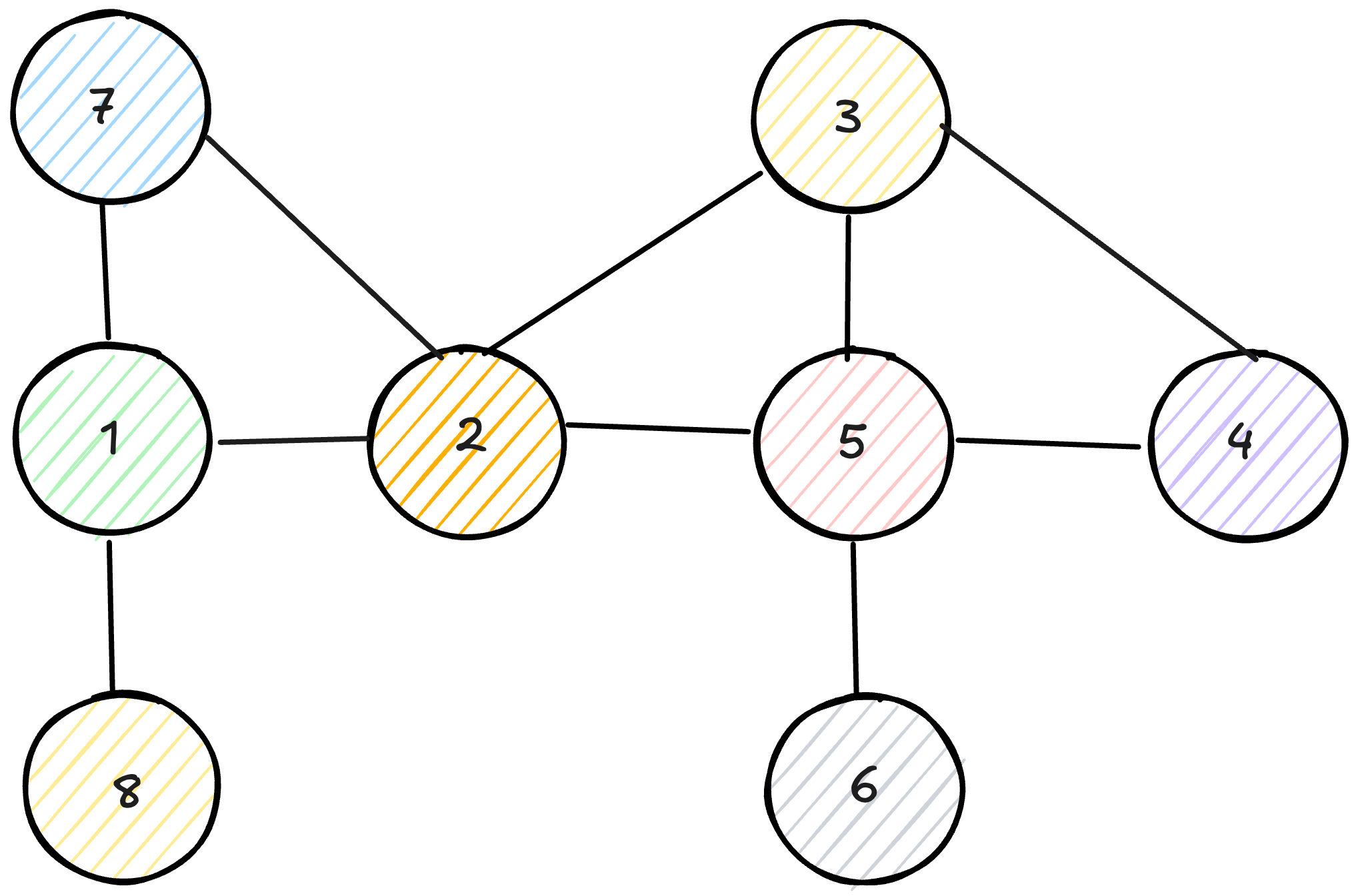
Let’s walk through an example using the graph with vertices (1-2), (1-7), (1-8), (2-3), (2-5), (3-4), (3-5), (4-5), (5-6).

Starting from vertex 1:

• Discover 1, explore its first neighbor 2

• Discover 2, explore its first neighbor 3

• Discover 3, explore its first neighbor 4

• Discover 4, explore its first neighbor 5

• Discover 5, explore its first neighbor 6

• Discover 6, all neighbors already discovered, backtrack to 5

• At 5, all neighbors discovered, backtrack to 4

• At 4, all neighbors discovered, backtrack to 3

• At 3, all neighbors discovered, backtrack to 2

• At 2, discover the remaining neighbor 7

• Discover 7, all neighbors already discovered, backtrack to 2

• At 2, all neighbors discovered, backtrack to 1

• At 1, discover the remaining neighbor 8

• Discover 8, all neighbors already discovered, backtrack to 1

• At 1, all neighbors discovered, done

The discovery order is 1, 2, 3, 4, 5, 6, 7, 8, which is very different from what BFS would produce. BFS would discover vertices in order of their distance from vertex 1, visiting 2, 7, and 8 before moving to 3, while DFS went as deep as possible before exploring other branches.

Similar to BFS, DFS builds a tree data structure as it explores the graph. Each time you discover a new vertex, you can record which vertex discovered it using a parent pointer. This creates a tree rooted at the starting vertex.

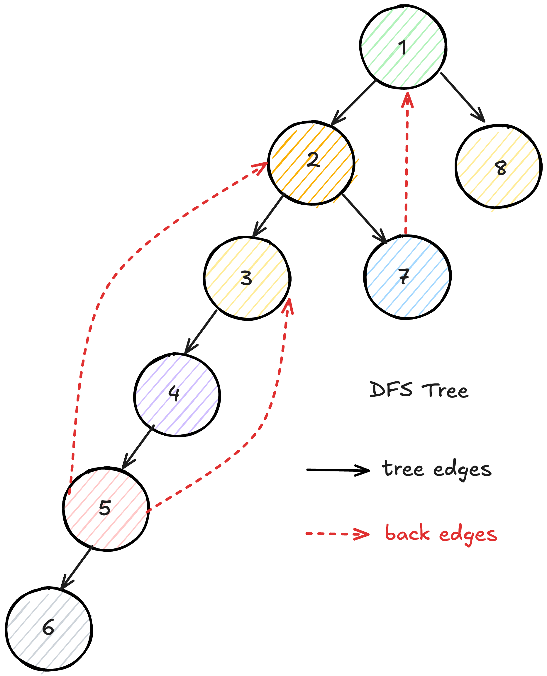
One subtle but important point: the order in which you examine neighbors matters. Different orderings can produce different DFS trees and different edge classifications, though tree and back edges remain consistent (the graph has the same shape). This is typically not a problem in practice because most DFS-based algorithms work correctly regardless of the specific ordering.

Key Properties of DFS

There are two properties of DFS worth knowing, as they provide valuable information about the graph’s structure: timestamps and edge classification.

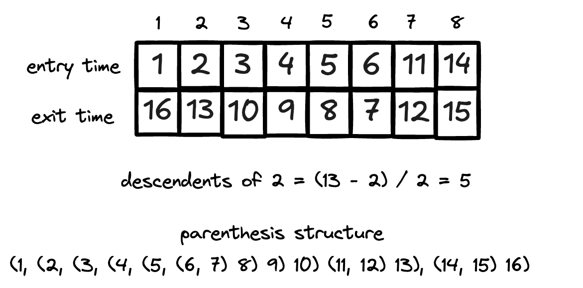
DFS maintains two important timestamps for each vertex: the discovery time (when you visit it for the first time and mark it as discovered) and the finishing time (when you have explored all its edges and marked it as processed). The time is initialized to zero and incremented by one every time one of these events occurs.

These timestamps follow a parenthesis structure. If you represent the discovery time of a vertex as an opening parenthesis and the finishing time as a closing parenthesis, the parentheses are properly nested. This property is helpful because it allows you to determine ancestor-descendant relationships simply by comparing timestamps. The descendants of a vertex u have timestamps that are nested within u's timestamp.

Indeed, for any two vertices u and v, one of three things must be true:

• Their time intervals are completely separate, and neither is an ancestor of the other in the DFS tree

• u’s interval is contained within v’s interval, so u is a descendant of v

• v’s interval is contained within u’s interval, so v is a descendant of u

In addition, the difference between a vertex’s finishing and discovery times tells you how many descendants it has. Since the clock ticks on each entry and exit, half this difference gives the descendant count.

The second interesting aspect of DFS is how it classifies edges. The type of each edge gives essential information about a graph and will be used in the algorithms discussed in the following sections. The classification depends on the type of graph.