


Hi Friends,
Welcome to the 200th issue of the Polymathic Engineer newsletter. This week, we continue our discussion of nearest neighbor search.
We have seen how to build a k-d tree: a binary search tree over points in which each node splits its region in two with a line through its point. This line alternates between vertical and horizontal at successive levels, with coordinate values lower than the threshold placed to the left, and values greater than or equal to the threshold placed to the right. Each node is associated with a rectangle in the plane, and the tree works for any number k of coordinates, although we draw k = 2.
We used this structure to identify the pickup point closest to a given delivery address: descend to the leaf containing the target, checking every node on the way, then backtrack, skipping every branch whose split line is farther than the best point found so far.
Every operation has an execution time that depends on the height of the tree. In this issue, we will look at how to keep that height small, what other information can be gathered from traversing the tree, and how fast all these operations are:
- Keeping the tree balanced
- Three more queries, one traversal
- How fast is nearest neighbor search
- Where k-d trees fall short
4,000+ AI Tools and Agents: How AWS Helps You Build
AWS resources for ISVs give software teams access to 4,000+ AI tools and agents through AWS Marketplace, alongside foundation models and services like Amazon Bedrock. Integrate AI into existing applications to support growth, build agentic workflows, and scale new capabilities across your customer base. Access the infrastructure, technical resources, and go-to-market support to take your next software innovation from development to market.
Sponsored by AWS
Keeping the tree balanced
So far we have consciously ignored a detail, a special characteristic we look for when it comes to binary search trees: whether the tree is balanced or not. As with any standard binary search tree (BST), the order in which we insert the points determines the shape of the tree.
In the previous issue, we carefully chose the points by hand to get a balanced tree, but it is easy to come up with a bad insertion sequence that would create an imbalanced tree. If the lockers lie along a highway running from northwest to southeast, and we insert them in that order, each new locker has a larger x and a smaller y than the previous one, so every insert goes right at the levels that split by x and left at the levels that split by y. The result is a zig-zag chain with linear height, and the regions it defines are a staircase of empty pieces nested into one corner of the map. Even with a random order, we have no guarantee that the tree ends up balanced.
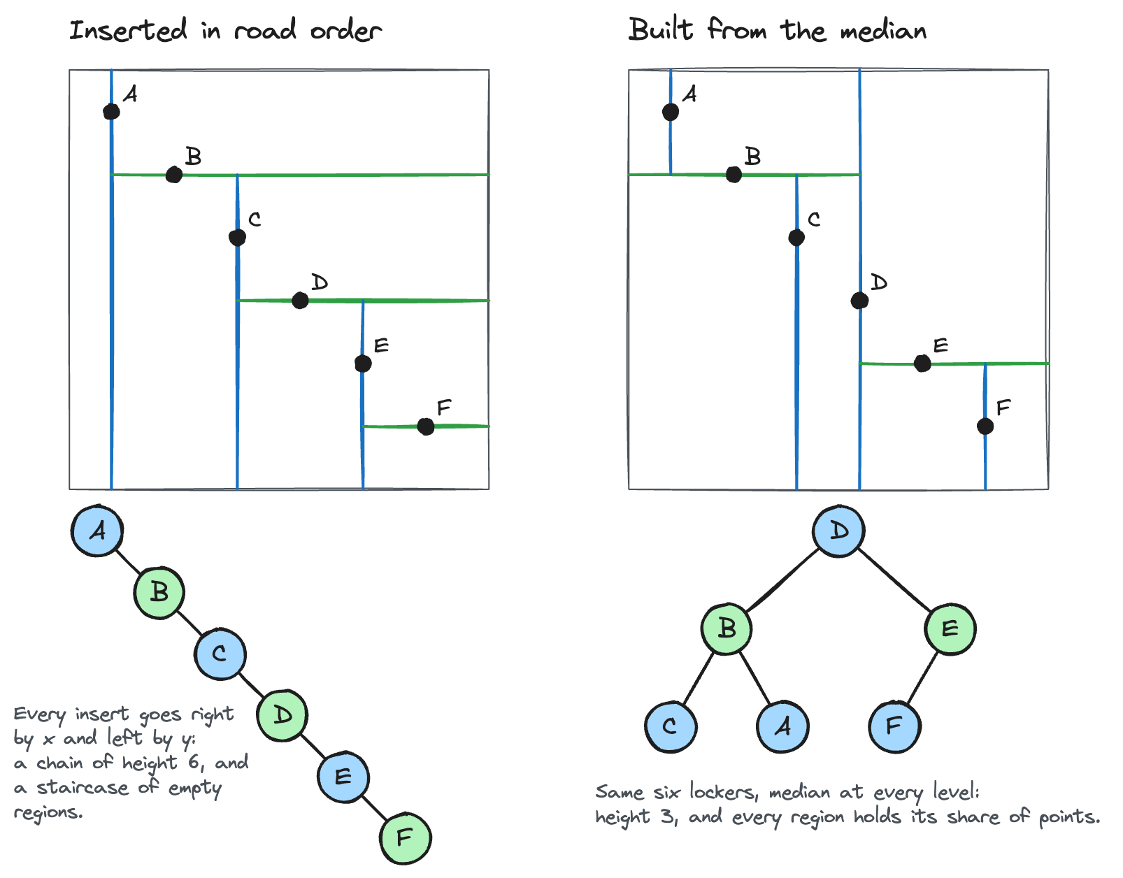
For regular BSTs, the solution involves rebalancing during insertion by means of rotations. Unfortunately, this is not a viable option for k-d trees. A rotation moves a subtree up or down one level, and the level decides the split coordinate, so every node in the moved subtree would end up splitting on the wrong coordinate. We would need to reevaluate every single node in the whole subtree and rebuild it, an operation that would inevitably require linear time.
Nevertheless, if we know the set of points in advance, we can determine an insertion order that produces a balanced tree. The principle is simple. Ideally, we would like the left and right subtrees of the root to have the same number of elements. To achieve that, we find the median of the points with respect to the first coordinate and use it as the root, so that half of the remaining points end up on the left branch and half on the right. Each branch is a k-d tree itself, so we repeat the same step on each half, with the caveat that this time we take the median with respect to the second coordinate, and so on for each level. Notice that we can’t just sort the array once and chunk it up into halves, because the sorting criterion changes at each level. The following code snippet builds a balanced tree this way.
def build(points, level=0):

    if not points:

        return None

    j = level % len(points[0])

    points = sorted(points, key=lambda p: p[j])

    mid = len(points) // 2

    while mid > 0 and points[mid - 1][j] == points[mid][j]:

        mid -= 1  # ties go right, as in search and insert

    node = KdNode(points[mid], level)

    node.left = build(points[:mid], level + 1)

    node.right = build(points[mid + 1:], level + 1)

    return node
What is the execution time of this construction? At each level, we find the median and partition the points around it, which takes linear time with a selection algorithm (sorting, as the code above does, adds a logarithmic factor), then make two recursive calls on half the points each. The resulting recurrence, T(n) = 2T(n/2) + O(n), has the well-known solution O(n log n). If we partition the array in place, the extra memory is only the O(n) needed for the tree. The important thing is that every split puts half the points on each side, no matter how they are distributed.
This method gives a balanced tree only if the tree does not change after construction, or if the number of points inserted and removed is negligible compared to the size of the tree.
Although delete is uncommon on a k-d tree, in any real-world application we’ll likely need to update our dataset, and removing a point makes things more complicated. The main issue is connected to how we find a replacement in the tree for the node we are going to remove.
When we delete an internal node, we must replace it with the minimum, on its split coordinate, of one of its subtrees, and finding that minimum requires visiting both branches at every level that splits on another coordinate. On a balanced tree, this takes O(n^(1-1/k)) time, which for k = 2 is O(√n): better than a full scan, but far from logarithmic.
Some k-d tree implementations don’t even offer a remove method. Since k-d trees are not self-balancing, they perform best when they are created with a static set of points, avoiding frequent insertion and removal. If the dataset changes, the common practice is to rebuild the tree in the background, once a sufficient number of points have been modified, and then replace the existing tree with the new version.
Three more queries, one traversal
While k-d trees were mainly designed to perform nearest neighbor search, they have proven particularly efficient for other kinds of operations.
For example: how to find the m closest points instead of a single one? Instead of a single distance, we need to keep track of the m shortest distances found so far and, at each step, use the m-th smallest distance to draw the circle and prune branches. A bounded priority queue (max-heap of size m) can take care of this: its top is the largest of the m distances kept, so a new point replaces the top only if it is closer, and the pruning radius is the top of the heap (infinity until we have found m points). Since Python’s heapq is a min-heap, we store distances as negative values:
import heapq

def m_nearest(node, target, m, heap=None):

    if heap is None:

        heap = []  # at most m entries of (-distance, point)

    if node is None:

        return heap

    d = distance(target, node.point)

    if len(heap) < m:

        heapq.heappush(heap, (-d, node.point))

    elif d < -heap[0][0]:

        heapq.heapreplace(heap, (-d, node.point))

    j = node.level % len(target)

    if target[j] < node.point[j]:

        close, away = node.left, node.right

    else:

        close, away = node.right, node.left

    m_nearest(close, target, m, heap)

    radius = math.inf if len(heap) < m else -heap[0][0]

    if abs(target[j] - node.point[j]) < radius:

        m_nearest(away, target, m, heap)

    return heap
Another interesting operation is finding points within a certain distance of a point of interest, such as all the lockers within 1 km of an address. This is a similar situation to the nearest neighbor search since we need to include all the points within a certain distance from a given point. However, we never update the radius: we start with the given distance, gather every point closer than that, and prune branches with the same test. The comparison becomes “less than or equal” if points exactly at the boundary count.
A third kind of operation is to check which points lie inside a rectangle aligned with the axes, such as all the lockers in the part of the map shown on the screen. Here the geometric interpretation is to query points whose coordinates are in certain ranges. Suppose that we are at a node that splits by y. We compare the node’s y with the rectangle's top and bottom, and there are three cases:
The split line falls inside the range; both branches may contain points of the rectangle, so we traverse both, and we report the node’s own point if its x is within range too.
The node’s y is above the top of the rectangle; every point in the right branch is higher still, so we only traverse the left branch.
The node’s y is below the bottom; we only traverse the right branch.
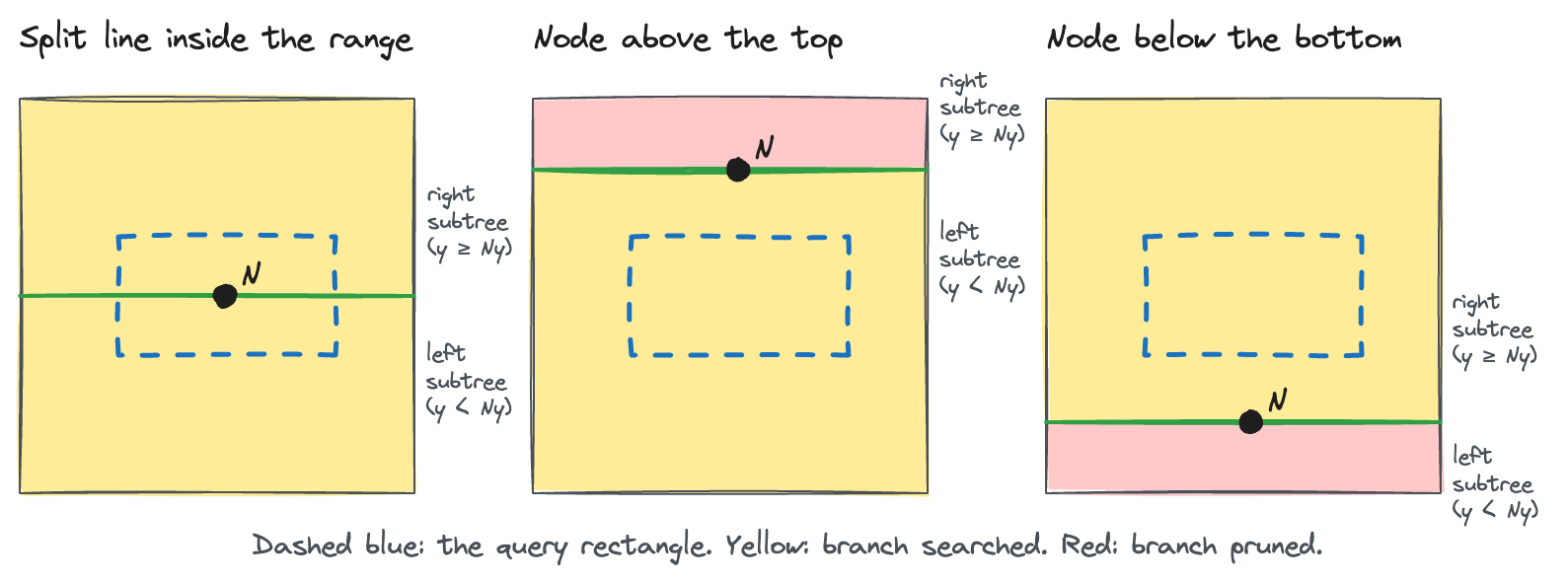
The same holds at the levels that split by x, checking the x coordinates instead. The following code snippet implements the search, with the rectangle given by its lowest and highest corners.
def range_search(node, lo, hi, found=None):

    if found is None:

        found = []

    if node is None:

        return found

    j = node.level % len(lo)

    if all(lo[i] <= node.point[i] <= hi[i] for i in range(len(lo))):

        found.append(node.point)

    if lo[j] < node.point[j]:  # part of the range lies left of the split line

        range_search(node.left, lo, hi, found)

    if node.point[j] <= hi[j]:  # part of the range lies right of the split line

        range_search(node.right, lo, hi, found)

    return found
This test works because each condition involves one coordinate at a time. If the conditions mix coordinates, the boundary of the region is a tilted line, and the shortcut of comparing a single coordinate with the split line is gone.
What is the execution time of these region searches? It heavily depends on the region. For a very small region intersecting only a single branch corresponding to a leaf, we prune every other branch and just follow a path to the leaf, so the execution time is O(log n) for a balanced tree. For a region large enough to contain all the points, we have to traverse the whole tree, and the execution time is O(n). Therefore, we can only say that the worst case is linear, even if the method prunes the tree whenever possible.
How fast is nearest neighbor search
Let’s start with the bad news. In the worst case, even for a balanced tree, we might have to traverse the whole tree before finding the nearest neighbor. Suppose that the lockers lie along a ring road around a city and the delivery address is right in the city center. Every locker is at the same distance from the address, so after the descent the circle passes through all of them, every split line falls within the circle, and virtually nothing is pruned. We end up visiting every node, exactly as in a brute-force search, so, unfortunately, the worst-case execution time for this query is O(n).
Luckily, there is also a silver lining. On a balanced tree with evenly distributed points, the average execution time is logarithmic in n, with a factor that grows exponentially with k: O(2^k + log n). The proof of this probabilistic bound is complex, and we won’t cover it here because it would require too much space. Nevertheless, it is worth understanding the intuition about why it works this way.
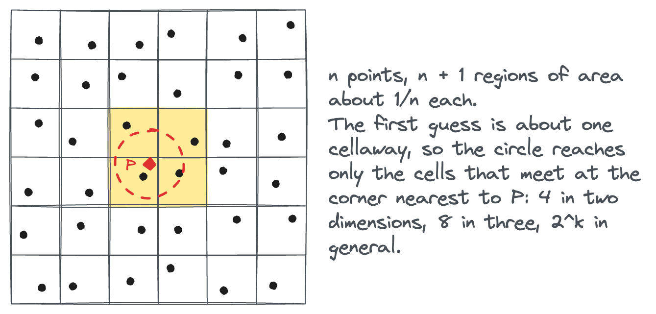
Consider a two-dimensional space: one point divides the plane into two regions, two points into three, three points will create four regions, and so on; in general, n points will create n+1 regions. If the tree is balanced and n is sufficiently large, we can assume these regions are approximately equally sized, so if the dataset covers a unit square, each region has an area of about 1/n and a side of about 1/√n.
When we run a nearest neighbor search, we first descend the tree from the root to the leaf whose region contains the target, which, for a balanced tree, means traversing O(log n) nodes. The point in that region is about 1/√n away, so the first guess is roughly that distance from the target. The next step is backtracking to visit all the regions within that distance. If the regions form something close to a regular grid, a circle of that radius around the target reaches the regions that meet at the grid corner closest to the target: four of them in two dimensions, eight in three, and 2^k in general. So, after finding the region where the target lies, we examine another O(2^k) regions, making the total execution time O(2^k + log n).
Let’s go through a numeric example. With a million lockers, the descent visits about 20 nodes, the backtracking checks a handful of neighboring regions, and we compute a few dozen distances in total, against a million for the brute-force loop.
While k is a constant for a given dataset, and we could in theory ignore it in the big-O analysis, in general k is considered a parameter, because we measure the performance of the method with respect to both the size and the dimension of the dataset. And for large values of k, 2^k becomes so big that it dominates the execution time: from k = 6 on, 2^k is larger than log n for any dataset we could store, so the execution time is effectively O(2^k). Roughly, the tree pays off only when n is well above 2^k. At k ≈ 20 we need a million evenly distributed points to break even, and at k ≈ 30 a billion. This is the curse of dimensionality: in high-dimensional spaces, data becomes very sparse, and the sphere around the target is very likely to intersect many branches in at least one dimension, so there is little left to prune.
Where k-d trees fall short
If we look back at our closest-locker problem, we started with nothing better than brute-force search, went through a few less-than-ideal attempts, and finally introduced k-d trees. They offer a major speed-up over a linear scan, yet they still have a few weak spots. Two of them we have already met. They are not self-balancing, so they perform best on a static set of points. And they become inefficient in high-dimensional spaces: a node with one child per quadrant ran out of memory at k = 100, and a k-d tree fits in memory at k = 100 but doesn’t help either, for a different reason.
The third weak spot is memory. K-d trees don’t work well with paged memory, because points are stored in the tree nodes: two lockers that are close on the map end up in nodes that may be far apart in memory, so a search touches many pages. Last but not least, they handle points well, but they can’t handle objects with a non-zero size, such as shapes.
To overcome these limitations, we could try a few approaches. We could use different criteria to decide where to split: choose at every step the coordinate with the greatest spread or variance rather than cycling through them, and divide the region into two halves instead of drawing the line through a point. Instead of storing one point per node, each node could describe a region and link to an array containing the actual points. Or we could settle for an approximate answer, stopping the backtracking early when the current best is good enough. The first two heuristics help on some datasets, but in general they don’t solve the issue with high-dimensional spaces. The third one does, at the cost of giving up an exact answer. After all, there are many cases where we can settle for a sub-optimal result. When we look for the document closest to a given article, or the product most similar to one that is no longer available, we are not even able to define a perfect distance.
Wrapping up
If you have read this far, you probably have a feeling for when a k-d tree is the right tool. Let’s make it explicit. For a static set of points defined by a small number of coordinates, a k-d tree built using the median is hard to beat; this solution is well-suited both to the case of pickup lockers and to most problems involving points on a map. Beyond that, we need new ways to partition the space, ideally trying to reduce sparsity. This is the path that leads to R-trees and SS-trees.